Ordinary Least Squares and Ridge Regression - Quick Tutorial

A visual comparison of Ordinary Least Squares (OLS) Variance & Ridge Regularization
Basic Linear Regression
Simplest way of trying to obtain an expected data value from previous data inputs is to assume a linear function. Take the various values of your data points, and try to minimize the distance between them and your linear equation.
Thanks to that simplicity, it has weights that can be easily understood. Compared to a lot of neural networks where thanks to the complex matrix calculations, trying to derive a meaning of the weights becomes intuitively more challenging.
The general linear regression has the format of:
Prediction = (slope * input) + interceptSciKit-Learn & OLS LinearRegression
Let us go over what we need to get a simple linear regression set up:
- Test Data Split into
- X_train, y_train: These are the values that will be given to the model to evaluate the slope and intercept
- X_test, y_test: These are the values that will be used when we have derived the slop and intercept from the first step to see how well our model performs
- LinearRegression model function from SciKit-Learn (sklearn)
For ease of use, we will be using the default diabetes database that comes built into the SciKit-Learn package.
1 - Setup & Data Loading
Load diabetes dataset
Extract only the third feature column
Split data into:
    - Training set (first portion)
    - Test set (last 20 samples)
2 - Train Model
Initialize Linear Regression model
Fit model to training data (X_train, y_train)
3 - Predict & Evaluate
Generate predictions for test set
Calculate:
    - Mean Squared Error between actual and predicted values
    - R² Score (how well predictions explain the variance)
Print both metrics
4 - Visualize Results
Create figure with 2 side-by-side plots

Left plot (Training Data)

Right plot (Test Data)

Display the figure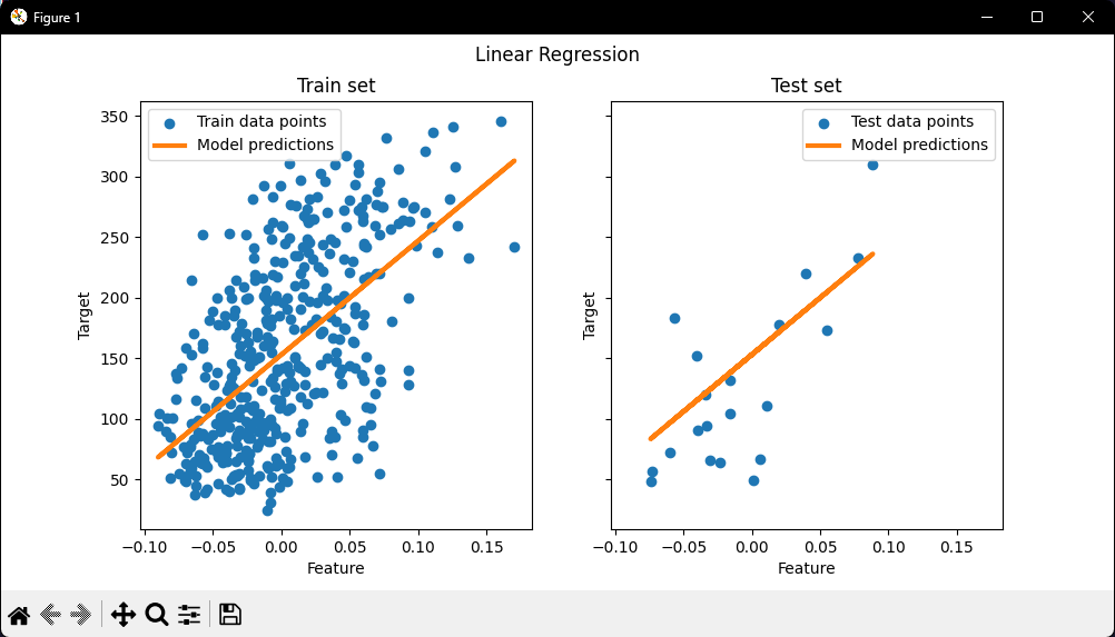
Note:
We can see how well (or poorly) it generalizes by looking at the R^2 score and mean squared error on the test set. In higher dimensions, pure OLS often overfits, especially if the data is noisy. Regularization techniques (like Ridge) can help reduce that.
Ridge Regression Variance
Next, we illustrate the problem of high variance more clearly by using a tiny synthetic dataset.
We sample only two data points, then repeatedly add small Gaussian noise to them and refit both OLS and Ridge. We plot each new line to see how much OLS can jump around, whereas Ridge remains more stable thanks to its penalty term.
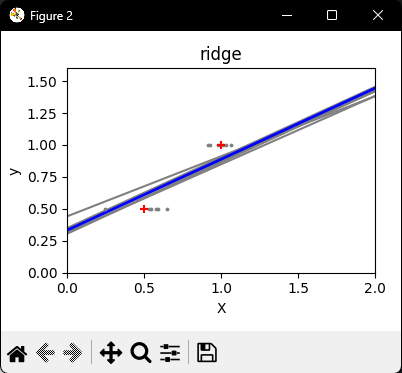
Ridge regression, reduces this variance by penalizing (shrinking) the coefficients, leading to more stable predictions.
The steps to follow for creating a Ridge Model is the exact same structure as the simple OLS.
1 - Setup & Data Prep
Create synthetic training data with 2 data points: (0.5, 0.5) and (1, 1)
Define test range from X=0 to X=2
2 - Define Models
Create two regression models:
    - OLS (Ordinary Least Squares)
    - Ridge (with penalty strength, alpha, of 0.1)
3 - Variance Simulation (Per Model)
For each model (OLS and Ridge):
    Create new figure

    Repeat 6 times:
        Add random noise to training data points
        Fit model on noisy data
4 - Plot & Display
Fit model on original clean training data (no noise)
Plot thick blue line showing final predictions
Plot red crosses showing original training points

Display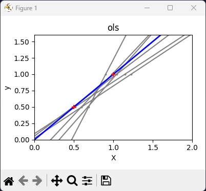
OLS vs Ridge Linear Regression Comparison.
Note:
OLS lines varied drastically each time noise was added, reflecting its high variance when data is sparse or noisy.
By contrast, Ridge regression introduces a regularization term (alpha = 0.1) that shrinks the coefficients, stabilizing predictions.
Conclusion
SciKit-Learn offers a wide variety of machine learning models with a wide range of applications: Classification, Regression, Clustering, Preprocessing, and many more.
I will be making more quick style pseudo-code tutorials that cover more of these packages as they are a great way to get a good introductory grasp over the material.
As always, the Python code will be in my GitHub repository: